Estimate the head probability of a coin
math/probability The problem
Toss a coin $T$ times. Let $X=\{x_1,\dots,x_T\} \in \{+,-\}^T$ be the result. Let $N_+ = \sum_{t=1}^T\mathbb I(x_t=+)$, $N_- = \sum_{t=1}^T\mathbb I(x_t=-)$. Let $P(x=+ \mid \theta)$ be the probability that the coin shows head in a toss. How to estimate $\theta$ from $X$?
MLE
\[\arg\max \log P(X \mid \theta) = \arg\max \big(N_+\log\theta + N_-\log(1-\theta)\big)\,.\]Taking derivative w.r.t. $\theta$ and letting it equal to zero yields
\[\theta = \frac{N_+}{N_+ + N_-}\,.\]As can be easily observed, it overfit when there’s not enough data(, e.g. when $N_+=6$, $N_-=0$).
MAP
Apply a beta prior $P(\theta \mid a, b) = \mathrm{Beta}(\theta \mid a, b)$. Set $a = b = 2$ so that it’s proper.
\[\arg\max \log P(\theta \mid X, a, b) = \arg\max \big(\log P(\theta \mid a, b) + \log P(X \mid \theta)\big)\,.\]Similarly, this yields
\[\theta = \frac{N_+ + a - 1}{N_+ + N_- + a + b - 2} = \frac{N_+ + 1}{N_+ + N_- + 2}\,.\]This is also called Laplace smoothing.
Full Bayesian
Apply a prior $P(\theta \mid a, b) = \mathrm{Beta}(\theta \mid a, b)$, and find the posterior:
\[P(\theta \mid X, a, b) = \frac{P(\theta \mid a, b) P(X \mid \theta)}{\int_0^1 P(\theta \mid a, b) P(X \mid \theta) \mathrm d \theta}\,.\]To address the integral, notice that
\[\int_0^1 x^\alpha (1-x)^\beta \mathrm dx = B(\alpha+1,\beta+1) = \frac{\Gamma(\alpha+1)\Gamma(\beta+1)}{\Gamma(\alpha+\beta+2)}\,,\]where $B(\cdot,\cdot)$ is the beta function, and $\Gamma(\cdot)$ is the gamma function. Therefore,
\[P(\theta \mid X, a, b) = \mathrm{Beta}(\theta \mid N_+ + a, N_- + b)\,.\]Now it’s straightforward to estimate the uncertainty in $\theta$ given $a$ and $b$.
Empirical Bayes
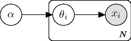
Here we abuse the term “empirical Bayes” since it original refers to a graphic model like this:
Whereas the model we are using is like this:
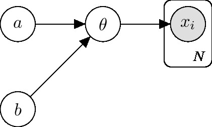
Since the derivation is similar (use of EM), we’ll continue with that notation.
Again, apply a beta prior $P(\theta \mid a, b)$, but now we regard $(a,b)$ as unknown parameters. By EM, the auxiliary function $Q$ is,
\[\log P(X \mid a, b) \ge Q(P, \tilde P) = \int_0^1 P(\theta \mid X, a^{(t-1)}, b^{(t-1)}) \log \tilde P(X, \theta \mid a, b) \mathrm d \theta\,,\]where at E-step, we have already computed $P(\theta \mid X, a^{(t-1)}, b^{(t-1)})$. Factorizing the logarithm,
\[\log \tilde P(X,\theta \mid a,b) = \log \tilde P(\theta \mid a,b) + \log \tilde P(X \mid \theta)\,,\]we notece that the second term on the r.h.s. does not rely on $a,b$. Therefore, we need only to optimize over the first term. So now the auxiliary function reduces to
\[\begin{aligned} Q(P, \tilde P) &= \int_0^1 P(\theta \mid X, a^{(t-1)},b^{(t-1)}) \log \tilde P(\theta \mid a, b)\\ &= \int_0^1 \mathrm{Beta}(\theta \mid N_+ + a^{(t-1)}, N_- + b^{(t-1)}) \log \mathrm{Beta}(\theta \mid a, b)\,.\\ \end{aligned}\]Taking partial derivative w.r.t. $a$ on both sides:
\[\begin{aligned} \frac{\partial Q}{\partial a} &= \frac{\partial}{\partial a} \int_0^1 \mathrm{Beta}(\theta \mid N_++a^{(t-1)},N_-+b^{(t-1)}) \log \mathrm{Beta}(\theta \mid a,b)\\ &= \frac{\partial}{\partial a}\int_0^1 \mathrm{Beta}(\theta \mid N_++a^{(t-1)},N_-+b^{(t-1)}) [(a-1)\log\theta + (b-1)\log(1-\theta) - \log B(a,b)] \mathrm d \theta\\ &= \int_0^1 \mathrm{Beta}(\theta \mid N_++a^{(t-1)},N_-+b^{(t-1)}) \frac{\partial}{\partial a} [(a-1)\log\theta + (b-1)\log(1-\theta) - \log B(a,b)] \mathrm d \theta\\ &= \int_0^1 \mathrm{Beta}(\theta \mid N_++a^{(t-1)},N_-+b^{(t-1)}) \left[\log\theta - \frac{\partial}{\partial a}\log B(a,b)\right] \mathrm d\theta\\ &= \int_0^1 \mathrm{Beta}(\theta \mid N_++a^{(t-1)},N_-+b^{(t-1)}) \log\theta \,\mathrm d\theta - \frac{\partial}{\partial a}\log B(a,b)\int_0^1 \mathrm{Beta}(\theta \mid N_++a^{(t-1)},N_-+b^{(t-1)}) \,\mathrm d\theta\\ &= \frac{1}{B(N_++a^{(t-1)},N_-+b^{(t-1)})} \int_0^1 \theta^{N_++a^{(t-1)}-1} (1-\theta)^{N_-+b^{(t-1)}-1} \log\theta \,\mathrm d\theta - \frac{\partial}{\partial a} \log B(a,b)\,.\\ \end{aligned}\]Notice that
\[\int_0^1 x^{\alpha-1} (1-x)^{\beta-1} \log x \,\mathrm d x = B(\alpha,\beta)(\psi(\alpha)-\psi(\alpha+\beta))\,,\]where $\psi(x) \triangleq \frac{\partial}{\partial x}\log\Gamma(x)$. We may using the same notation $\psi$ to expand the log-derivative of beta function. Thus,
\[\frac{\partial Q}{\partial a} = \psi(N_++a^{(t-1)})-\psi(N_++a^{(t-1)}+N_-+b^{(t-1)}) - (\psi(a) - \psi(a+b))\,.\]Similarly,
\[\frac{\partial Q}{\partial b} = \psi(N_-+b^{(t-1)}) - \psi(N_++a^{(t-1)}+N_-+b^{(t-1)}) - (\psi(b)-\psi(a+b))\,.\]Setting initial value $a^{(0)}=b^{(0)}=1$, we may find optimal solution for $a$ and $b$.
BUT REALLY, here we may compute directly $\log P(X \mid a, b)$ due to the conjugate beta prior!
It turns out that
\[L(a,b) \triangleq \log P(X \mid a, b) = \log\frac{B(N_++a,N_-+b)}{B(a,b)}\,.\]Hence,
\[\begin{cases} \frac{\partial L}{\partial a} = \psi(N_++a) + \psi(a+b) - \psi(a) - \psi(N_++N_-+a+b)\\ \frac{\partial L}{\partial b} = \psi(N_-+b) + \psi(a+b) - \psi(b) - \psi(N_++N_-+a+b)\\ \end{cases}\]Coding time:
import numpy as np
from scipy.special import digamma, betaln
from scipy.optimize import minimize

# the log-likelihood
def fun(x, p, n):
    a, b = x
    # the minus sign is because we are doing gradient descent (not ascent)
    return -(betaln(p + a, n + b) - betaln(a, b))

def jac(x, p, n):
    a, b = x
    # the minus sign is because we are doing gradient descent (not ascent)
    ja = -(digamma(p + a) + digamma(a + b) - digamma(a)
           - digamma(p + n + a + b))
    jb = -(digamma(n + b) + digamma(a + b) - digamma(b)
           - digamma(p + n + a + b))
    return np.array([ja, jb])

# Suppose N+ = 6 and N- = 0:
print(minimize(fun, np.ones(2), args=(6, 0), method='L-BFGS-B', jac=jac,
               bounds=[(1e-10, None), (1e-10, None)]))
The optimization result is:
message: CONVERGENCE: NORM_OF_PROJECTED_GRADIENT_<=_PGTOL
  success: True
   status: 0
      fun: 1.6934720292738348e-10
        x: [ 1.817e+00  1.000e-10]
      nit: 2
      jac: [-5.917e-11  1.693e+00]
     nfev: 3
     njev: 3
 hess_inv: <2x2 LbfgsInvHessProduct with dtype=float64>
From the result, the mean of the prior distribution goes to 1.0 (from left), the mode does not exists, and the density at 1.0 goes to infinity. Such prior will drive $\theta$ to 1. We observe that the model has severly overfit, exactly the same case if we were using simple MLE.
Conclusion
In conclusion, data-driven approach to set hyperparameters (e.g. empirical Bayes) (, at least in this example,) works only when there are enough well-sampled data.