Estimate the expectation of the function of a random variable
math/probability First prepare the functions we’ll use later. The implementations can be tested by py.test.
# %load expectation_of_function.py
from functools import partial

import numpy as np
from scipy.special import logsumexp
from scipy import stats


def softmax(x):
    b = np.max(x, axis=-1, keepdims=True)
    z = np.exp(x - b)
    return z / np.sum(z, axis=-1, keepdims=True)


def softmax_jac(x):
    s = softmax(x)
    I = np.eye(x.shape[0])
    return s[:, np.newaxis] * (I - s[np.newaxis, :])


def test_softmax_jac():
    n, d = 100, 100
    X = np.random.randn(n, d)
    I = np.eye(d)
    for j in range(n):
        s = softmax(X[j])
        expected = np.empty((d, d))
        for k in range(d):
            expected[k] = s[k] * (I[k] - s)
        assert np.allclose(softmax_jac(X[j]), expected)


def softmax_hess(x):
    s = softmax(x)
    a1 = np.outer(s, s) - np.diag(s)
    a2 = np.eye(x.shape[0]) - s[np.newaxis, :]
    a3 = np.matmul(a2[:, :, np.newaxis], a2[:, np.newaxis, :])
    a4 = a1[np.newaxis, :, :] + a3
    return s[:, np.newaxis, np.newaxis] * a4


def test_softmax_hess():
    n, d = 100, 100
    X = np.random.randn(n, d)
    I = np.eye(d)
    for j in range(n):
        s = softmax(X[j])
        expected = np.empty((d, d, d))
        for k in range(d):
            expected[k] = s[k] * (
                np.outer(s, s) - np.diag(s) + np.outer(I[k] - s, I[k] - s))
        assert np.allclose(softmax_hess(X[j]), expected)


def logsoftmax(x):
    return x - logsumexp(x, axis=-1, keepdims=True)


def logsoftmax_jac(x):
    s = softmax(x)
    I = np.eye(x.shape[0])
    return I - s[np.newaxis, :]


def logsoftmax_hess(x):
    s = softmax(x)
    return (np.outer(s, s) - np.diag(s))[np.newaxis]


# Deprecated
def expectation_logsoftmax_approx_at_mu(mu, Sigma):
    s = softmax(mu)
    ls = logsoftmax(mu)
    return ls + np.trace(np.matmul(np.outer(s, s) - np.diag(s), Sigma)) / 2


def sigmoid(x):
    z = np.where(x >= 0, np.exp(-x), np.exp(x))
    return np.where(x >= 0, 1 / (1 + z), z / (1 + z))


def test_sigmoid():
    n = 1000
    x = np.random.randn(n)
    expected = [sigmoid(x[j]) for j in range(n)]
    assert np.allclose(sigmoid(x), expected)


def sigmoid_jac(x):
    z = sigmoid(x)
    return z * (1 - z)


def sigmoid_hess(x):
    z = sigmoid(x)
    return z * (1 - z) * (1 - 2 * z)


def logsigmoid(x):
    return -np.logaddexp(0, -x)


def logsigmoid_jac(x):
    return 1 - sigmoid(x)


def logsigmoid_hess(x):
    z = sigmoid(x)
    return z * (z - 1)


# pylint: disable=too-many-arguments
def expectation_approx(mu, Sigma, a, fun, jac, hess):
    f = fun(a)
    J = jac(a)
    H = hess(a)
    d = mu - a
    if f.ndim == 1:
        a1 = f
        a2 = np.dot(J, d)
        a3 = np.ravel(
            np.matmul(
                np.matmul(d[np.newaxis, np.newaxis, :], H), d[np.newaxis, :,
                                                              np.newaxis]))
        a4 = np.trace(np.matmul(H, Sigma[np.newaxis]), axis1=1, axis2=2)
        return a1 + a2 + (a3 + a4) / 2
    a1 = f
    a2 = np.dot(J, d)
    a3 = np.dot(np.dot(d, H), d)
    a4 = np.dot(H, Sigma)
    if a4.ndim > 0:
        a4 = np.trace(a4)
    return a1 + a2 + (a3 + a4) / 2


def test_expectation_approx():
    n, d = 100, 100
    mu = np.random.randn(n, d)
    Sigma = np.random.randn(n, d, d)
    Sigma = np.matmul(Sigma, np.transpose(Sigma, (0, 2, 1)))
    for j in range(n):
        actual = expectation_approx(mu[j], Sigma[j], mu[j], logsoftmax,
                                    logsoftmax_jac, logsoftmax_hess)
        expected = expectation_logsoftmax_approx_at_mu(mu[j], Sigma[j])
        assert np.allclose(actual, expected)


def expectation_MC(fun, rvs, n):
    X = rvs(size=n)
    return np.mean(fun(X), axis=0)


def multivariate_normal_rvs(mean, cov):
    return partial(stats.multivariate_normal.rvs, mean=mean, cov=cov)


def gamma_rvs(a, b):
    return partial(stats.gamma.rvs, a=a, scale=1 / b)


def gamma_mean(a, b):
    return a / b


def gamma_mode(a, b):
    return (a - 1) / b


def gamma_cov(a, b):
    return a / b**2


def dirichlet_rvs(alpha):
    return partial(stats.dirichlet.rvs, alpha=alpha)


def dirichlet_mean(alpha):
    alpha0 = np.sum(alpha)
    return alpha / alpha0


def dirichlet_mode(alpha):
    K = alpha.shape[0]
    alpha0 = np.sum(alpha)
    return (alpha - 1) / (alpha0 - K)


def dirichlet_cov(alpha):
    K = alpha.shape[0]
    alpha0 = np.sum(alpha)
    return (np.eye(K) * alpha * alpha0 - np.outer(alpha, alpha)) / (
        alpha0**2 * (alpha0 + 1))
from matplotlib import pyplot as plt
We’d like to estimate $\mathbb E_{\boldsymbol x \sim p_X(\boldsymbol x)}[f(\boldsymbol x)]$. The idea is to approximate the expectation by the 2nd-order Taylor expansion.
Assume that the Tayler series is expanded at $\boldsymbol x = \boldsymbol a$:
\[\begin{aligned} f(\boldsymbol x) &= f(\boldsymbol a) + \nabla f(\boldsymbol a)^\top(\boldsymbol x-\boldsymbol a) + \frac{1}{2}(\boldsymbol x-\boldsymbol a)^\top\mathbf H f(\boldsymbol a)(\boldsymbol x-\boldsymbol a)+R_2(\boldsymbol x)\\ \mathbb E[f(\boldsymbol x)] &\approx f(\boldsymbol a) + \nabla f(\boldsymbol a)^\top (\boldsymbol\mu-\boldsymbol a) + \frac{1}{2}\big((\boldsymbol\mu-\boldsymbol a)^\top \mathbf H f(\boldsymbol a) (\boldsymbol\mu-\boldsymbol a) + \operatorname{tr}(\mathbf H f(\boldsymbol a) \boldsymbol\Sigma)\big)\,,\\ \end{aligned}\]with error bound (see definition here; and Little-o notation here):
\[\begin{aligned} R_2(\boldsymbol x) &\in o(\|\boldsymbol x-\boldsymbol a\|^2)\\ \mathbb E[R_2(\boldsymbol x)] &\in o(\|\boldsymbol\mu-\boldsymbol a\|^2 + \operatorname{tr}(\boldsymbol\Sigma))\,.\\ \end{aligned}\]It seems that if the Tayler series is not expanded at the mean, the error bound will increase.
Give it a try on $\mathbb E_{x \sim \text{Exp}(\lambda)}[\log\operatorname{sigmoid}(x)]$, where $\text{Exp}(\lambda)$ is the exponential distribution, or Gamma distribution with parameter $a=1$. The Monte Carlo result is taken as the groundtruth:
a, b = 1, 1
expected = expectation_MC(logsigmoid, gamma_rvs(a, b), 100000)
approx_at_mu = expectation_approx(gamma_mean(a, b), gamma_cov(a, b), gamma_mean(a, b),
                                  logsigmoid, logsigmoid_jac, logsigmoid_hess)
approx_at_mode = expectation_approx(gamma_mean(a, b), gamma_cov(a, b), gamma_mode(a, b),
                                    logsigmoid, logsigmoid_jac, logsigmoid_hess)
np.abs(approx_at_mu - expected), np.abs(approx_at_mode - expected)
(0.025421238663924095, 0.05700076508490559)
Okay, so we’d better expand the Taylor series at mean.
So now the expectation approximation reduces to
\[\mathbb E[f(\boldsymbol x)] \approx f(\boldsymbol\mu) + \frac{1}{2}\operatorname{tr}(\mathbf H f(\boldsymbol\mu) \boldsymbol\Sigma)\,,\]by plugging in $\boldsymbol a=\boldsymbol\mu$, and with error bound
\[R_2(\boldsymbol x) \in o(\operatorname{tr}(\boldsymbol\Sigma))\,.\]We may now verify that the error is indeed positively related to the trace of the covariance. Take the approximation of $\mathbb E_{\boldsymbol x \sim \mathcal N(\boldsymbol\mu,\boldsymbol\Sigma)}[\log\operatorname{softmax}(\boldsymbol x)]$ as an example, and again regards the Monte Carlo result as the groundtruth:
d = 50
mu = np.random.randn(d)
Sigma = np.random.randn(d, d)
# make the covariance positive semi-definite
Sigma = np.dot(Sigma.T, Sigma)

expected = expectation_MC(logsoftmax, multivariate_normal_rvs(mu, Sigma), 100000)
approx = expectation_approx(mu, Sigma, mu, logsoftmax, logsoftmax_jac, logsoftmax_hess)
np.trace(Sigma), np.mean(np.abs(approx - expected))
(2534.8991641540433, 11.581681866513225)
Sigma /= 1000

expected = expectation_MC(logsoftmax, multivariate_normal_rvs(mu, Sigma), 100000)
approx = expectation_approx(mu, Sigma, mu, logsoftmax, logsoftmax_jac, logsoftmax_hess)
np.trace(Sigma), np.mean(np.abs(approx - expected))
(2.5348991641540435, 0.0006679801955036791)
The mean error drops by 25000 times as the trace decreases by 1000 times.
Now take $\mathbb E_{\boldsymbol x \sim \text{Dirichlet}(\boldsymbol\alpha)}[\log\operatorname{softmax}(\boldsymbol x)]$ as another example:
d = 5
alpha = 6 / d * np.ones(d)
mu = dirichlet_mean(alpha)
Sigma = dirichlet_cov(alpha)

expected = expectation_MC(logsoftmax, dirichlet_rvs(alpha), 100000)
approx = expectation_approx(mu, Sigma, mu, logsoftmax, logsoftmax_jac, logsoftmax_hess)
np.trace(Sigma), np.mean(np.abs(approx - expected))
(0.11428571428571428, 0.0005659672760450097)
d = 5
alpha = 60 / d * np.ones(d)
mu = dirichlet_mean(alpha)
Sigma = dirichlet_cov(alpha)

expected = expectation_MC(logsoftmax, dirichlet_rvs(alpha), 100000)
approx = expectation_approx(mu, Sigma, mu, logsoftmax, logsoftmax_jac, logsoftmax_hess)
np.trace(Sigma), np.mean(np.abs(approx - expected))
(0.013114754098360656, 0.0001473556430732881)
The mean error drops three times as the trace decreases by ten times.
Hence, the error is certainly positively related to the trace of the covariance.
To conclude the notebook, assuming that the underlying distribution is multivariate Gaussian, let’s see if the approximation conforms to intuition when $f$ is sigmoid or softmax – to see if the expectation fails within the range of sigmoid or softmax.
mu = np.array(1.7)
Sigma = np.logspace(-7, 2, 10)
approxes = np.array([expectation_approx(mu, Sigma[j], mu, sigmoid, sigmoid_jac, sigmoid_hess)
                     for j in range(Sigma.shape[0])])
expected = np.array([expectation_MC(sigmoid, multivariate_normal_rvs(mu, Sigma[j]), 100000)
                     for j in range(Sigma.shape[0])])
fig, ax = plt.subplots()
ax.plot(Sigma, approxes, marker='o', label='approximation')
ax.plot(Sigma, expected, linestyle='--', color='red', label='groundtruth')
ax.set_xlabel(r'$\operatorname{tr}(\Sigma)$')
ax.set_xscale('log')
ax.legend()
ax.grid()
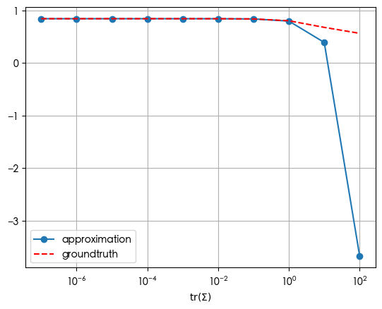
For sigmoid, after the trace of the covariance exceeds 1.0, the approximation starts to deviate from the groundtruth.
d = 384
mu = np.random.randn(d)
Sigma = np.random.randn(d, d)
Sigma = np.dot(Sigma.T, Sigma)
a = np.logspace(0, 7, 8)[::-1]
approxes = np.stack([expectation_approx(mu, Sigma / a[j], mu, softmax, softmax_jac, softmax_hess)
                     for j in range(a.shape[0])])
expected = np.stack([expectation_MC(softmax, multivariate_normal_rvs(mu, Sigma / a[j]), 100000)
                     for j in range(a.shape[0])])
traces = np.trace(Sigma[np.newaxis] / a[:, np.newaxis, np.newaxis], axis1=1, axis2=2)
fig, ax = plt.subplots()
ax.plot(traces, np.mean(approxes, axis=1), color='blue', alpha=0.8, marker='o', label='approximation')
ax.fill_between(traces, np.max(approxes, axis=1), np.min(approxes, axis=1), color='blue', alpha=0.2)
ax.plot(traces, np.mean(expected, axis=1), color='red', alpha=0.8, linestyle='--', label='groundtruth')
ax.fill_between(traces, np.max(expected, axis=1), np.min(expected, axis=1), color='red', alpha=0.2)
ax.set_xlabel(r'$\operatorname{tr}(\Sigma)$')
ax.set_xscale('log')
ax.legend()
ax.grid()
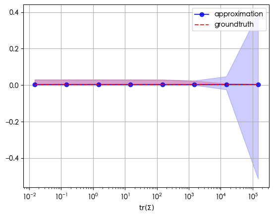
For softmax, after the trace of the covariance exceeds 1000, the range of the expectation starts to be counterintuitive.